TurboQuant: Google’s Breakthrough in Efficient Large Language Model KV Cache Management Promises Unprecedented Compression Without Accuracy Loss
The intricate workings of Large Language Models (LLMs) have long been attributed to a core mechanism known as "attention," the conceptual brain that allows these powerful AI systems to discern relationships between different parts of the input data. This attention mechanism, operating on Query (Q), Key (K), and Value (V) components, is fundamental to the impressive capabilities of modern LLMs. However, the computational demands of attention, particularly during the inference phase where new tokens are generated, present a significant challenge. For every new token, the Key and Value matrices for all preceding tokens are recalculated, leading to a repetitive and computationally expensive process.
To address this inefficiency, the concept of a KV cache was introduced. By storing the calculated Key and Value matrices in Video RAM (VRAM), subsequent computations could reuse this cached information, dramatically reducing inference latency. This innovation has become a standard practice across virtually all major LLM architectures. Yet, the widespread adoption of the KV cache has introduced its own set of problems, primarily concerning memory overhead. For smaller language models (SLMs), this additional memory burden might be negligible, but for the rapidly growing "mega-LLMs" with billions of parameters, it translates into substantial VRAM consumption, often consuming an additional 20-30% of the total memory. This overhead is not static; it escalates with longer context windows and a greater number of concurrent users, as each user session necessitates its own independent KV cache.
Researchers have explored various avenues to mitigate this growing memory issue, including Grouped-Query Attention (GQA) and techniques like PagedAttention, as well as quantization methods reducing model precision to 4-bit or 8-bit. While these approaches have offered improvements in memory efficiency, they have consistently come at the cost of compromised accuracy, a trade-off that has been difficult to overcome. Until now.
A groundbreaking development from Google, detailed in a recent pre-print paper, introduces TurboQuant, a novel solution that appears to achieve significant KV cache compression without sacrificing model accuracy. The researchers behind TurboQuant claim it not only addresses the memory overhead but also achieves a theoretically optimal balance between compression and performance for this class of problem.
The Two-Stage Power of TurboQuant
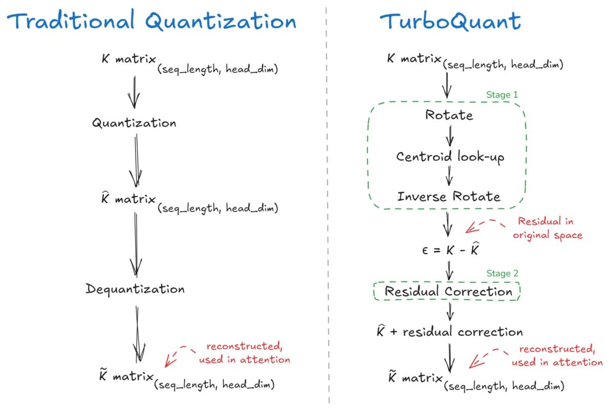
TurboQuant employs a sophisticated two-stage process: PolarQuant and Residual Correction. This sequential approach is what sets it apart from traditional quantization methods.

Stage 1: PolarQuant – Compressing the Core
The first stage, PolarQuant, focuses on compressing the Key and Value matrices. This involves two key operations: Rotation and Lloyd-Max Quantization.
The Challenge of Outliers in Quantization: Traditional quantization methods often struggle with outliers – extremely large or small values within a dataset. Consider a 4-dimensional key vector for a token, such as [0.125, 0.103, 0.220, 6.030]. In attention mechanisms, such outlier values are not uncommon. When a quantizer with a limited range of discrete levels is applied to this vector, the massive spike of 6.030 forces the quantizer to stretch its capacity, inevitably leading to a significant loss of information across all dimensions. The resulting quantized vector might be something like [0, 0, 0, 1], rendering most of the original data meaningless.
Rotation for Isotropic Distribution: PolarQuant tackles this problem head-on by first applying a rotation to the vector. This rotation, performed using a random orthogonal matrix (y = R*x), effectively "spins" the vector in high-dimensional space. The effect is to redistribute the energy of the outlier values across the other dimensions, smoothing out the distribution and making it more uniform or "isotropic." While the individual values within the vector change, its overall magnitude remains constant. The example vector [0.125, 0.103, 0.220, 6.030], after rotation, might transform into a more balanced representation like [1.42, -0.85, 2.31, 0.97].
This rotation process pushes the distribution of vector coordinates towards a Gaussian-like form. More precisely, the rotated vector becomes uniformly distributed on the unit sphere, a property that, according to the central limit theorem, implies that each coordinate, when squared and normalized by the total energy, follows a Beta distribution:
where ‘d’ represents the head dimension. This statistical property is rooted in multivariate statistics, where the ratio of independent chi-squared distributed variables follows a Beta distribution.
Lloyd-Max Quantization for Optimal Encoding: Following the rotation, the second key operation in PolarQuant is Lloyd-Max Quantization. This algorithm is designed to minimize the mean squared error (MSE) by intelligently placing quantization levels (centroids). Essentially, it’s an optimized form of clustering for one-dimensional data. For a rotated vector, such as [1.42, -0.85, 2.31, 0.97], if we were performing 1-bit quantization, Lloyd-Max would determine the optimal threshold to divide the data into two groups, minimizing the overall error. The statistical insight here is that the value which minimizes squared error for a group of points is their mean.

A crucial advantage of this approach is that due to the consistent distribution (Beta) established by the rotation, the optimal quantization codebook can be precomputed offline. This means that instead of recalculating quantization levels for every new vector during inference, a fixed codebook, dependent only on the head dimension (d) and the number of bits (b), can be reused. This precomputation significantly speeds up the quantization process.
The quantized values are not stored as floating-point numbers but as indices (idx) into these precomputed codebooks. For example, if a codebook has 8 levels, the values are stored as indices 0 through 7, requiring 3 bits per value. It’s important to note that in TurboQuant’s PolarQuant stage, the actual stored index uses ‘b-1’ bits per dimension, leaving room for the subsequent residual correction stage.
During dequantization, when the Key matrix is needed for attention calculations, these indices are looked up in the codebook to retrieve the corresponding float values. This dequantized matrix is then transformed back into the original space using the transpose of the rotation matrix. The residual error, defined as the difference between the original Key matrix and the dequantized matrix (µ = Original K matrix – K_dequantized matrix), is then calculated, setting the stage for the second phase.
Stage 2: Residual Correction – Recovering Lost Information
The second stage of TurboQuant focuses on capturing the essence of the information lost during the compression in PolarQuant, rather than discarding it. It addresses the residuals (µ) generated in Stage 1 by asking focused questions about their characteristics.
Quantized Johnson-Lindenstrauss (QJL) Transform: TurboQuant employs a Quantized Johnson-Lindenstrauss (QJL) Transform. This involves multiplying the residual vector (µ) with a random projection matrix (S) of shape (d, d). The critical information extracted here is the sign of the resulting values (+1 or -1). These sign projections, mathematically represented as Sign(µ * S), capture the directional information of the residual. The randomness of the matrix S is not arbitrary; the Johnson-Lindenstrauss lemma guarantees that such random projections preserve the inner product structure of the data with high probability.
However, signs alone only indicate direction and not magnitude. To compensate for this, TurboQuant also stores the L2 norm (magnitude) of the residual vector (||µ||) as a single scalar value per vector. This scalar is crucial for restoring the correct magnitude during the reconstruction process.

Reconstruction and Scaling: During dequantization, the stored sign bits are multiplied back with the transposed S matrix. This result is then scaled by a specific factor: (sqrt(π/2) / d). This scaling factor, derived from mathematical analysis, is essential to correct any bias introduced by the sign-based estimation of the inner product, ensuring an unbiased reconstruction. The full formula for the QJL-reconstructed component is:
Finally, the dequantized matrix from Stage 1 (K_dequantized) and the QJL-reconstructed residual (K_QJL) are added together to produce the fully reconstructed Key matrix (K_reconstructed = K_dequantized + K_QJL).
Performance Metrics and Implications
The results presented by the TurboQuant research team are striking. The paper reports a KV cache compression of over 4.5x to 5x, translating to an effective 3.5 to 2.5 bits per channel. Crucially, this level of compression is achieved with near-zero loss in accuracy, meaning the performance of LLMs using TurboQuant is practically indistinguishable from those operating with full-precision KV caches. This stands in stark contrast to previous quantization techniques, which often saw significant accuracy degradation.
The implications of TurboQuant are profound, particularly in the context of the ongoing push for longer context windows in LLMs. As models become capable of processing and remembering vast amounts of information over extended sequences, the KV cache bottleneck becomes increasingly critical. TurboQuant offers a pathway to alleviate this pressure without demanding additional hardware resources. By optimizing how KV cache data is stored and accessed, it can enable larger models to run more efficiently on existing hardware, potentially democratizing access to advanced AI capabilities.
The ability to compress KV caches so effectively without accuracy loss could also lead to:
- Faster Inference: Reduced memory bandwidth requirements and smaller data sizes can translate directly into quicker response times for LLM applications.
- Increased Model Capacity: More memory can be allocated to model parameters or larger context windows, leading to more sophisticated and capable LLMs.
- Reduced Energy Consumption: Less data movement and fewer computations can lead to lower power consumption, making AI deployment more sustainable.
- Wider Deployment: The ability to run larger models on less powerful hardware could enable their use in a broader range of devices and applications, from edge computing to consumer-grade hardware.
The Future of KV Cache Management
The introduction of TurboQuant marks a significant milestone in the ongoing quest for efficient LLM inference. It demonstrates that by rethinking the fundamental principles of data representation and reconstruction, substantial gains in performance and memory efficiency can be achieved without compromising the core capabilities of these models.

While the research paper provides a detailed mathematical framework, the core insight is a shift in focus: instead of striving for perfect reconstruction of every numerical value, TurboQuant concentrates on preserving the essential information that the attention mechanism actually requires. This pragmatic approach, coupled with a robust mathematical foundation, positions TurboQuant as a potentially transformative technology in the LLM landscape.
The question now is whether this innovation will become the new standard for KV cache management, effectively closing a significant chapter in LLM optimization, or serve as a foundational element for even more advanced techniques to come. As the field continues to evolve, the efficiency and effectiveness of solutions like TurboQuant will be paramount in unlocking the full potential of artificial intelligence.
Related Posts

Unlocking Engineering Efficiency: A Deep Dive into Anthropic’s Claude Cowork for Enhanced Productivity
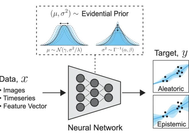
Uncertainty Quantification in Machine Learning: A Deep Dive into Evidential Deep Learning and Deep Evidential Regression