

The Critical Role of Context Payload Optimization in In-Context Learning for Tabular Foundation Models
The past couple of years have witnessed a significant surge in investment and development within the domain of tabular foundation models, encompassing both open-source and commercial offerings. These models are increasingly built around the principle of "in-context learning" (ICL), a paradigm shift from traditional supervised machine learning. A prime example of this evolution is SAP’s release of the SAP-RPT-1 suite of models in 2025. These models are specifically engineered to tackle enterprise resource planning (ERP)-centric tasks, including financial planning, sales and procurement order processing, and supply chain management. Unlike conventional supervised learning, where models require extensive, task-specific training and fine-tuning, ICL enables a single, broadly pretrained model to adapt dynamically. This adaptation occurs by leveraging relatively small amounts of task-specific data provided within a "context payload," which effectively functions as an ephemeral training set during inference.
While this move towards ICL significantly reduces the need for the costly and time-consuming retraining of task-specific tabular models, it introduces a critical trade-off at inference time: the balance between accuracy and latency. This challenge is particularly pronounced for centrally hosted models, such as the SAP-RPT-1. On one hand, the time expended in transmitting the context payload to the model server, and subsequently for the model to interpret and learn from this data, directly contributes to the overall response latency. Naturally, smaller payloads tend to reduce this latency. On the other hand, the model often needs to infer complex data schemas and understand diverse data distributions from heterogeneous contextual data. This data can frequently contain outliers, missing values, and long-tail patterns, all of which can impede accurate predictions. Consequently, achieving high predictive accuracy typically necessitates larger, meticulously curated context payloads. In practice, this creates a pressing need to devise strategies for distilling the context payload to minimize response times without compromising the model’s predictive performance. Further complicating matters are secondary trade-offs involving model service throughput, response stability, and the economic cost associated with model usage. These multifaceted challenges underscore why "context payload optimization" has emerged as a central architectural concern in workflows powered by ICL.
This article delves deeper into the inference-time trade-offs inherent in ICL-based tabular foundation models. It outlines practical strategies for optimizing context payloads and demonstrates the efficacy of KNN-based context prefiltering as a payload optimization technique through an end-to-end Python example.
Inference-Time Trade-Offs: The Iron Triangle of AI
A robust framework for analyzing the inference-time trade-offs associated with ICL-based tabular foundation models is the "iron triangle" concept. This framework, previously discussed in the context of AI product development, highlights the inherent tensions users must navigate between response quality, inference cost, and latency. It serves as an inference-time analog to the classic project management "triple constraint" of scope, time, and cost. The fundamental principle is that improving one aspect of this triangle often exerts pressure on the others. For instance, delivering higher-quality responses typically requires more computational resources, thereby increasing both latency and cost. Conversely, efforts to reduce latency may necessitate sacrificing some quality or incurring higher expenses for faster hardware. Similarly, lowering costs often leads to slower or less accurate AI responses.
This triangular tension is acutely felt in the realm of ICL-based tabular foundation models. The primary challenge lies in balancing response quality, often measured by metrics like precision and recall, against latency. Consider a real-time fraud detection system deployed at ATMs. Both precision (minimizing false positives) and speed are paramount, yet optimizing for one can negatively impact the other, particularly in how the context payload is constructed. Larger, more comprehensive payloads provide the AI model with a richer set of examples from which to infer underlying schemas, identify rare or long-tail patterns, and ultimately deliver more accurate predictions. However, each additional row or feature increases the volume of data that must be transmitted to the model server and processed during inference, introducing a measurable overhead to the end-to-end response time. In time-sensitive applications, even a marginal increase in payload size can noticeably degrade system responsiveness, potentially leading to a diminished user experience.
Beyond this primary trade-off, several secondary considerations emerge in practical deployments. A larger context payload not only extends inference time but also consumes more "tokens" – a unit of data often used for billing in large language models and foundation models. This creates a direct tension between response latency and the monetary cost of model usage, a concern that is particularly salient for centrally hosted services like SAP-RPT-1. Furthermore, increased payload size can augment the per-request compute time, introducing a latency-throughput trade-off that may compel AI system development teams to make difficult scaling decisions. There’s also a potential for a quality-stability trade-off: while increasing the volume and variety of contextual data can enhance predictive accuracy, it may also reduce output determinism by introducing noise and making predictions more sensitive to minor variations in the input data. Finally, employing more sophisticated payload selection methods, such as KNN-based retrieval, can indeed improve prediction quality but simultaneously escalates payload construction time, adding to the overall latency.
Context Payload Optimization Strategies
Strategies for optimizing context payloads can be broadly categorized along two orthogonal dimensions: the "method" and the "moment" of optimization. The method dictates how the payload is curated – the specific filtering, clustering, or embedding techniques employed to compress the raw context data. The moment of optimization, conversely, addresses when and where this curation takes place. This includes whether it is precomputed offline or derived dynamically at inference time, and whether the optimization is performed by the client application or the model service itself. The choice of the moment for constructing the optimized payload can significantly impact inference latency and system maintainability. Ultimately, the chosen method and moment of payload optimization should align with the specific use case’s scope, budget constraints, latency thresholds, and quality requirements.
Methods of Optimization
Payload optimization methods can be further divided into task-agnostic and task-aware approaches. Task-agnostic methods, such as random sampling and recency-based sampling, do not require prior knowledge of the specific prediction task or the semantic structure of the data. Random sampling is straightforward to implement, fast, and generally unbiased, making it a useful baseline or fallback strategy. However, it risks inadvertently discarding data points that capture rare yet crucial patterns essential for optimal model performance. Recency-based sampling, which assumes the presence of timestamps in the data, retrieves the most recent records. This can be beneficial for datasets with time-bound distributions (e.g., seasonality) or those susceptible to temporal drift. Yet, this method often overlooks the broader dataset structure and may overemphasize short-term noise. In essence, task-agnostic methods offer simplicity and speed but provide limited control over the representativeness and relevance of the resultant payload.
In contrast, task-aware methods leverage information about the prediction task, the query data, and the underlying data distribution to select the most pertinent records for the context payload. A common task-aware technique is K-nearest neighbors (KNN) sampling, which identifies historical data records that are semantically similar to the query records. This approach can yield highly relevant contextual data and demonstrate strong empirical performance. However, it necessitates defining distance metrics (e.g., cosine similarity) and often requires auxiliary models for data vectorization or embedding, making it computationally intensive at scale. Another class of techniques utilizes clustering algorithms (e.g., K-means, hierarchical clustering, DBSCAN) to extract representative samples from clusters associated with the query data. This can ensure adequate coverage of diverse data patterns while minimizing redundancy, although it typically involves offline cluster computation and periodic recomputation to maintain cluster relevance.
More sophisticated task-aware methods are also emerging. For instance, both the raw context and query data can be embedded into a low-dimensional vector space – encoded within the API request and decoded in the response. This effectively acts as a form of lossy compression, sacrificing some accuracy in exchange for reduced latency and cost due to a smaller payload. Retrieval-augmented generation (RAG) techniques can further enhance the payload by incorporating domain-specific grounding information, thereby boosting response relevance. In summary, while task-aware methods generally yield higher-quality context payloads, they come with a greater engineering and computational overhead.
Moments of Optimization
A key decision regarding the "moment" of optimization concerns whether some payload curation steps can be performed offline. For example, a "golden" dataset can be pre-curated from historical data, optimized for informational density, and enriched with metadata like cluster IDs or hashtags. Relevant records can then be efficiently selected from this leaner, golden dataset to construct and transmit the context payload at inference time. Golden datasets are particularly well-suited for applications with stable schemas and repetitive tasks, such as auto-completion of common sales orders in ERP systems. However, their curation and ongoing maintenance can introduce additional overhead for development teams. Conversely, on-the-fly optimization derives the payload dynamically at inference time, based on the current query data and available historical records. This approach is more adaptive but can increase the computational cost and latency for each individual inference call. It’s also worth noting that on-the-fly optimization doesn’t necessarily reduce development team overhead; the savings from not maintaining a golden dataset might be offset by the prompt engineering efforts required for dynamic context payload optimization.
Another moment-related decision pertains to whether optimization occurs on the client or the service side. Client-side optimization grants the consuming application complete control, enabling custom preprocessing, local caching, and more straightforward debugging. However, it also places the burden of implementing and maintaining optimization logic on each individual client, potentially leading to duplicated efforts across applications and teams. Client-side processing also demands sufficient client-side computational resources, which can be a constraint for applications running on resource-limited IoT or edge devices. Service-side optimization, on the other hand, benefits from economies of scale. With sufficient usage across multiple clients, an AI service provider can justify deploying more sophisticated algorithms and higher-end hardware than any single client might independently adopt. The provider can also leverage deep, model-specific expertise and gain insights into model performance across various client environments – compounding over time – to develop a more refined and harmonized optimization strategy. Service-side processing also simplifies governance, as software updates, privacy controls, audit logging, and compliance checks can be enforced uniformly. The downsides include reduced transparency for clients, increased load on the provider’s infrastructure, and the ongoing cost for the AI service provider to develop and maintain the optimization logic.
Naturally, ICL-based tabular AI workflows can also adopt a hybrid strategy, combining the strengths of different approaches. A practical pattern involves coarse client-side filtering to reduce the payload to a manageable size, perhaps by selecting the top-K nearest neighbors or applying other simple heuristics. This is then paired with fine-grained service-side pruning using model-aware signals to refine the final context before inference. Hybrid approaches can strike an effective balance between transparency, flexibility, governance, and overall performance.
Hands-On Demo: KNN-Based Context Prefiltering
To illustrate the practical application of context payload optimization, we will employ the Solar Flare dataset and a playground version of the SAP-RPT-1 model. This demonstration will utilize KNN-based context prefiltering to optimize the payload.
Setup
First, ensure you have the necessary Python packages installed. Create a requirements.txt file with the following content:
pandas
numpy
requests
scikit-learn
ucimlrepo
Then, install these dependencies using pip: pip install -r requirements.txt.
Next, create a Python file (e.g., demo.py) and begin by adding the following import statements:
import pandas as pd
import numpy as np
import time
import json
import requests
import sys
import os
from datetime import datetime
from sklearn.preprocessing import LabelEncoder
from sklearn.metrics import pairwise_distances
from ucimlrepo import fetch_ucirepo
Following the imports, configure the experiment parameters:
EXPERIMENT_ORDER = ["without_prefiltering", "with_prefiltering"]

API_URL = "https://rpt.cloud.sap/api/predict"
ACCESS_TOKEN_PATH = "access_token.json"  # File containing your API token

# Load API token from the specified JSON file
with open(ACCESS_TOKEN_PATH, "r") as f:
    token = json.load(f)["access_token"]

n_test_rows = 20  # Number of query rows to use for testing
mask_proportion = 0.3  # Proportion of column values to mask (simulating a prediction scenario)
max_masked_columns = 4  # Playground model limitation on masked columns
random_seed = 3  # Seed for reproducibility
rng = np.random.default_rng(random_seed)  # Initialize random number generator

ctx_max_rows = 600  # Maximum number of rows allowed in the context window
To enable comprehensive logging of the script’s output, including console messages and saved logs, implement the following Tee class and initialization:
class Tee(object):
    """A simple stdout tee: Prints to console and writes to a log file."""
    def __init__(self, logfile_path):
        self.terminal = sys.stdout
        self.log = open(logfile_path, "a", encoding="utf-8")

    def write(self, message):
        self.terminal.write(message)
        self.log.write(message)

    def flush(self):
        self.terminal.flush()
        self.log.flush()

script_dir = os.path.dirname(os.path.abspath(__file__))

timestamp = datetime.now().strftime("%Y%m%d_%H%M%S")

log_filename = f"log_knn_seedrandom_seed_''.join([x[0] for x in EXPERIMENT_ORDER])_timestamp.log"

log_path = os.path.join(script_dir, log_filename)

sys.stdout = Tee(log_path)

print(f"Logging enabled. Output is being written to: log_pathn")
The subsequent sections will introduce helper functions for diagnostic reporting, constructing the SAP-RPT-1 model payload, safely interacting with the model API, and exporting prediction results to a CSV file.
A function to compute feature statistics of the dataset:
def compute_feature_stats(df, random_seed):
    """
    Computes cardinality and HHI concentration metric for each feature.
    Saves results to: feature_stats_knn_seed<seed>_<timestamp>.csv
    """
    stats = []

    for col in df.columns:
        if col == "id":
            continue

        cardinality = df[col].nunique()

        # Normalized value counts
        vc = df[col].value_counts(normalize=True)

        # Herfindahl-Hirschman Index (HHI)
        # HHI = 1.0 implies perfect concentration (only one value appears)
        # HHI = 0.01 implies a very uniform distribution
        # A higher HHI indicates greater feature concentration
        hhi = float((vc ** 2).sum())

        # Dominant category proportion (share of the most common feature value)
        max_prop = float(vc.max())

        stats.append(
            "feature": col,
            "cardinality": cardinality,
            "hhi": hhi,
            "max_proportion": max_prop
        )

    stats_df = pd.DataFrame(stats)

    timestamp = datetime.now().strftime("%Y%m%d_%H%M%S")
    filename = f"feature_stats_knn_seedrandom_seed_timestamp.csv"

    stats_df.to_csv(filename, index=False)
    print(f"Saved feature stats to filenamen")
Functions for simulating the prediction scenario, constructing the SAP-RPT-1 model payload, and safely invoking the model API:
def mask_row_values(row, allowed_mask_columns, p, rng):
    """Masks a proportion of values in a row with '[PREDICT]'."""
    row = row.copy()
    mask_candidates = [c for c in allowed_mask_columns if rng.random() < p]
    for c in mask_candidates:
        row[c] = "[PREDICT]"
    return row

def build_payload(df, index_column="id"):
    """Builds the payload dictionary for the SAP-RPT-1 API."""
    return "rows": df.to_dict(orient="records"), "index_column": index_column

def safe_call_rpt1(payload, token):
    """Safely calls the SAP-RPT-1 API and handles potential errors."""
    headers =
        "Content-Type": "application/json",
        "Authorization": f"Bearer token"


    try:
        response = requests.post(API_URL, json=payload, headers=headers)

        try:
            response_json = response.json()
        except ValueError:
            print("nNon-JSON response from RPT-1:")
            print(response.text)
            return False, "error": "Non-JSON response"

        if "error" in response_json:
            print("nRPT-1 API returned an error:")
            print(json.dumps(response_json, indent=2))
            return False, response_json

        if "aiApiResponsePayload" not in response_json:
            print("nMissing aiApiResponsePayload:")
            print(json.dumps(response_json, indent=2))
            return False, response_json

        payload = response_json["aiApiResponsePayload"]

        if "predictions" not in payload:
            print("nMissing predictions in aiApiResponsePayload:")
            print(json.dumps(response_json, indent=2))
            return False, response_json

        return True, response_json

    except requests.exceptions.RequestException as e:
        print("nHTTP request failed:")
        print(str(e))
        return False, "error": str(e)
Functions for post-processing predictions:
def flatten_predictions(pred_list):
    """Flattens the nested prediction structure into a more usable DataFrame."""
    flat =
    for entry in pred_list:
        row =
        for key, value in entry.items():
            if key == "id":
                row["id"] = str(value)
            else:
                if isinstance(value, list) and len(value) > 0:
                    row[key] = value[0].get("prediction")
                else:
                    row[key] = None
        flat[row["id"]] = row
    return pd.DataFrame(flat.values()).set_index("id")

def evaluate_accuracy(pred_df, true_df, masked_df):
    """Evaluates the prediction accuracy against true values for masked columns."""
    correct = 0
    total = 0
    for idx in masked_df.index:
        for col in masked_df.columns:
            # Only count predictions for columns that were originally masked
            if masked_df.loc[idx, col] == "[PREDICT]":
                total += 1
                if pred_df.loc[idx, col] == true_df.loc[idx, col]:
                    correct += 1
    return correct, total, correct / total if total > 0 else np.nan

def export_predictions_dynamic(true_rows, masked_rows, pred_df, filename):
    """
    Exports a CSV file with predictions, filling masked columns with model outputs
    and retaining original values for unmasked columns.
    """
    # Ensure pred_df is indexed by id and matches the type of true_rows index
    pred_df = pred_df.copy()
    pred_df.index = pred_df.index.astype(str) # Align index type

    # Reindex pred_df to match true_rows for proper alignment
    pred_df = pred_df.reindex(true_rows.index)

    # Start with the true rows
    merged = true_rows.reset_index().copy()

    # Align mask by id
    masked_by_id = masked_rows.copy()

    # Dynamically add prediction columns
    for col in pred_df.columns:
        pred_col = f"pred_col"

        # Initialize with true values
        merged[pred_col] = merged[col]

        # Overwrite only where the original value was masked
        mask = masked_by_id[col] == "[PREDICT]"
        # Ensure indices align for assignment
        merged.loc[mask.values, pred_col] = pred_df.loc[mask.values, col]

    # Save the merged DataFrame to CSV
    merged.to_csv(
        filename,
        index=False,
        encoding="utf-8",
        quoting=1
    )

    print(f"Saved results to filenamen")
Now, load and prepare the Solar Flare dataset:
solar_flare_data = fetch_ucirepo(id=89)

df = pd.concat([solar_flare_data.data.features, solar_flare_data.data.targets], axis=1)

# Assign meaningful column names
df.columns = [
    "zurich_class",
    "spot_size",
    "spot_dist",
    "activity",
    "evolution",
    "prev24_fac",
    "hist_complex",
    "region_complex",
    "area",
    "area_largest_spot",
    "c_class",
    "m_class",
    "x_class",
]

# Ensure an 'id' column exists for tracking rows
if "id" not in df.columns:
    df["id"] = df.index.astype(str)

# Convert numeric codes to words to force categorical behavior and handle potential ambiguities
replacement_map = "0": "zero", "1": "one", "2": "two", "3": "three"
for col in df.columns:
    if col != "id":
        df[col] = df[col].astype(str)
        df[col] = df[col].replace(replacement_map)
Save the computed feature statistics:
compute_feature_stats(df, random_seed)Simulate the prediction scenario. First, split the Solar Flare dataset into context and query/test rows:
df_test_rows = df.sample(n=n_test_rows, random_state=random_seed).reset_index(drop=True)

df_context_full = df.drop(df_test_rows.index).reset_index(drop=True)
Next, randomly mask some columns in the query/test rows to mimic a scenario where the model needs to predict missing values:
all_columns = [c for c in df.columns if c != "id"]

# Select columns to be masked
allowed_mask_columns = rng.choice(all_columns, size=max_masked_columns, replace=False)

df_test_rows_masked = df_test_rows.apply(
    lambda row: mask_row_values(row, allowed_mask_columns, mask_proportion, rng),
    axis=1
)

df_test_rows_masked["id"] = df_test_rows["id"] # Re-assign IDs after masking
Prefiltering Logic
The following code implements the KNN-based prefiltering to derive an optimized set of context rows (df_context_prefiltered):
start_prefilter = time.time()

n_test = df_test_rows.shape[0]
# Calculate budget for KNN neighbors per test row to stay within context window limit
budget_per_row = max(1, (ctx_max_rows - n_test) // n_test)

print(f"Context max rows: ctx_max_rows")
print(f"Number of test rows: n_test")
print(f"KNN budget per test row: budget_per_rown")

# Encode categorical features using LabelEncoder for distance calculations.
# In a production scenario, more sophisticated vectorizers or embedding models could be used.
encoders =
df_context_enc = df_context_full.copy()
df_test_enc = df_test_rows.copy()

for col in df_context_full.columns:
    if col == "id":
        continue
    le = LabelEncoder()
    # Fit on context data and transform both context and test data
    df_context_enc[col] = le.fit_transform(df_context_full[col].astype(str))
    df_test_enc[col] = le.transform(df_test_rows[col].astype(str))
    encoders[col] = le

# Convert encoded dataframes to numpy arrays for efficient distance computation
X_context = df_context_enc.drop(columns=["id"]).to_numpy()
X_test = df_test_enc.drop(columns=["id"]).to_numpy()

selected_indices = []
# For each test row, find its nearest neighbors in the full context
for x_test in X_test:
    # Compute pairwise distances between the test row and all context rows
    dists = pairwise_distances([x_test], X_context)[0]
    # Get indices of the 'budget_per_row' nearest neighbors
    nearest = np.argsort(dists)[:budget_per_row]
    selected_indices.extend(nearest)

# Create the prefiltered context by selecting unique nearest neighbors and resetting index
df_context_prefiltered = (
    df_context_full.iloc[selected_indices]
    .drop_duplicates()
    .reset_index(drop=True)
)

end_prefilter = time.time()
prefilter_time = end_prefilter - start_prefilter

print(f"Prefiltering time: prefilter_time:.3f seconds")
print(
    f"Prefiltered rows: len(df_context_prefiltered) "
    f"(100 * len(df_context_prefiltered) / len(df_context_full):.2f% of full context)n"
)
Running Experiments
The following functions orchestrate the model calls, both with and without the KNN-based context optimization:
def run_without_prefiltering():
    """
    Runs the experiment without any context payload optimization.
    The full context and masked test rows are sent directly.
    """
    print("=== CASE 1: NO PREFILTERING ===")

    start = time.time()

    # Combine full context with masked test rows
    df_context_without_prefiltering = pd.concat(
        [df_context_full, df_test_rows_masked], ignore_index=True
    )

    payload = build_payload(df_context_without_prefiltering)

    # Call the RPT-1 API
    success, response = safe_call_rpt1(payload, token)

    end = time.time()

    inference_time = end - start
    print(f"Case 1 inference time: inference_time:.3f seconds")

    accuracy = np.nan
    if success:
        # Flatten predictions and evaluate accuracy
        pred_df = flatten_predictions(response["aiApiResponsePayload"]["predictions"])
        pred_df = pred_df.astype(str) # Ensure consistent data type for comparison

        true_rows = df_test_rows.set_index("id")
        masked_rows = df_test_rows_masked.set_index("id")

        correct, total, accuracy = evaluate_accuracy(pred_df, true_rows, masked_rows)
        print(f"Case 1 accuracy: correct/total = accuracy:.3fn")

        # Export results
        timestamp = datetime.now().strftime("%Y%m%d_%H%M%S")
        filename = f"results_knn_seedrandom_seed_c_timestamp.csv"
        export_predictions_dynamic(true_rows, masked_rows, pred_df, filename)

    else:
        print("Skipping accuracy evaluation due to API error.n")

    return inference_time, accuracy

def run_with_prefiltering():
    """
    Runs the experiment with KNN-based context prefiltering.
    The optimized context and masked test rows are sent.
    """
    print("=== CASE 2: KNN-BASED PREFILTERING ===")

    start = time.time()

    # Combine prefiltered context with masked test rows
    df_context_with_prefiltering = pd.concat(
        [df_context_prefiltered, df_test_rows_masked], ignore_index=True
    )

    payload = build_payload(df_context_with_prefiltering)

    # Call the RPT-1 API
    success, response = safe_call_rpt1(payload, token)

    end = time.time()

    inference_time = end - start
    print(f"Case 2 inference time (RPT-1 call): inference_time:.3f seconds")

    accuracy = np.nan
    if success:
        # Flatten predictions and evaluate accuracy
        pred_df = flatten_predictions(response["aiApiResponsePayload"]["predictions"])
        pred_df = pred_df.astype(str) # Ensure consistent data type for comparison

        true_rows = df_test_rows.set_index("id")
        masked_rows = df_test_rows_masked.set_index("id")

        correct, total, accuracy = evaluate_accuracy(pred_df, true_rows, masked_rows)
        print(f"Case 2 accuracy: correct/total = accuracy:.3fn")

        # Export results
        timestamp = datetime.now().strftime("%Y%m%d_%H%M%S")
        filename = f"results_knn_seedrandom_seed_t_timestamp.csv"
        export_predictions_dynamic(true_rows, masked_rows, pred_df, filename)

    else:
        print("Skipping accuracy evaluation due to API error.n")

    return inference_time, accuracy
Finally, execute the experiments and present the results:
def run_experiments(order):
    """Runs experiments in the specified order and collects results."""
    results =
    for exp in order:
        if exp == "without_prefiltering":
            results["without_prefiltering"] = run_without_prefiltering()
        elif exp == "with_prefiltering":
            results["with_prefiltering"] = run_with_prefiltering()
        else:
            print(f"Unknown experiment type: exp")
    return results

print("=== RUNNING EXPERIMENTS ===n")
results = run_experiments(EXPERIMENT_ORDER)

print("n=== FINAL RESULTS ===")
print(results)
It is important to note that the initial API call to the model service may exhibit a longer execution time. This is often due to "warm-up" processes, which can include loading the model into memory, initializing runtime environments, and establishing network connections. Subsequent calls typically benefit from this initialized state, leading to faster response times. Modifying the order of experiments in EXPERIMENT_ORDER will alter which experiment absorbs this initial warm-up cost. Experimenting with different orders can reveal performance differences influenced by this factor.
The Wrap
As ICL-based tabular foundation models gain broader adoption, the focus of optimization is shifting from traditional supervised model training to the sophisticated construction of context payloads. The performance characteristics of an ICL-based system—in terms of quality, cost, and latency—are becoming less dependent on the foundational model’s training regimen and far more influenced by how effectively the context payload is utilized during inference. This paradigm shift is likely to drive organizations towards establishing repeatable and reusable patterns for managing these context payloads. Just as the industry has seen standardization around feature stores, data pipelines, and prompt engineering conventions, we can anticipate a similar consolidation of best practices for context payload design. Over time, these established patterns could become integral to the shared vocabulary of development teams working with ICL-based tabular foundation models, elevating context optimization to a primary architectural concern.


Related Posts

Unlocking Engineering Efficiency: A Deep Dive into Anthropic’s Claude Cowork for Enhanced Productivity
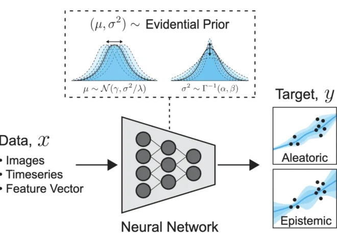
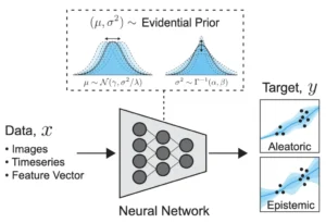
Uncertainty Quantification in Machine Learning: A Deep Dive into Evidential Deep Learning and Deep Evidential Regression

